


Introduction
A journey of thousand miles begin with a single step. In a similar way, the journey of mastering machine learning algorithms begins ideally with Regression. It is simple to understand, and gets you started with predictive modeling quickly. While this ease is good for a beginner, I always advice them to also understand the working of regression before they start using it.
Lately, I have seen a lot of beginners, who just focus on learning how to perform regression (in R or Python) but not on the actual science behind it. I am not blaming the beginners alone. Here is a script from a 2 day course on machine learning:
Running regression in Python and R doesn’t take more than 3-4 lines of code. All you need to do is, pass the variables, run the script and get the predicted values. And congratulations! You’ve run your first machine learning algorithm.
The course literally spends no time even explaining this simple algorithm, but covers neural networks as part of the course. What a waste of resources!
So, in this article, I’ve explained regression in a very simple manner. I have covered the basics, so that you not only understand what is regression and how it works, but also how to compute the popular R² and the science behind it.
Just a word of caution, you can’t use it all types of situation. Simple regression has some limitations, which can be overcome by using advanced regression techniques.

The D Hack – Double Prize Money – Registrations Open Now
What is Linear Regression?
Linear Regression is used for predictive analysis. It is a technique which explains the degree of relationship between two or more variables (multiple regression, in that case) using a best fit line / plane. Simple Linear Regression is used when we have, one independent variable and one dependent variable.
Regression technique tries to fit a single line through a scatter plot (see below). The simplest form of regression with one dependent and one independent variable is defined by the formula:
Y = aX + b
Let’s understand this equation using the scatter plot below:

Above, you can see that a black line passes through the data points. Now, you carefully notice that this line intersects the data points at coordinates (0,0), (4,8) and (30,60). Here’s a question. Find the equation that describe this line? Your answer should be:
Y= a * X + b
Now, find the value of a and b?
With out going in its working, the outcome after solving these equations is:
a = 2, b = 0
Hence, our regression equation becomes: Y= 2*X + 0 i.e. Y= 2*X
Here, Slope = 8/4 =2 or 60/30 =2 and Intercept = 0 (as Y =0 when x is 0). So, equation would be
Y = 2*X + 0
This equation is known as linear regression equation, where Y is target variable, X is input variable. ‘a’ is known as slope and ‘b’ as intercept. It is used to estimate real values (cost of houses, number of calls, total sales etc.) based on input variable(s). Here, we establish relationship between independent and dependent variables by fitting a best line. This best fit line is known as regression line and represented by a linear equation Y= a *X + b.
Now, you might think that in above example, there can be multiple regression lines those can pass through the data points. So, how to choose the best fit line or value of co-efficients a and b.
Let’s look at the methods to find the best fit line.
How to find the best regression line?
We discussed above that regression line establishes a relationship between independent and dependent variable(s). A line which can explain the relationship better is said to be best fit line.
In other words, the best fit line tends to return most accurate value of Y based on X i.e. causing a minimum difference between actual and predicted value of Y (lower prediction error). Make sure you understand the image below.

Here are some methods which check for error:
- Sum of all errors (∑error)
- Sum of absolute value of all errors (∑|error|)
- Sum of square of all errors (∑error^2)
Let’s evaluate performance of above discussed methods using an example. Below I have plotted three lines (y=2.3x+4, y=1.8x+3.5 and y=2x+8) to find the relationship between y and x.
Table shown below calculates the error value of each data point and the total error value (E) using the three methods discussed above:

After looking at the table, the following inferences can be generated:
- Sum of all errors (∑error): Using this method leads to cancellation of positive and negative errors, which certainly isn’t our motive. Hence, it is not the right method.
- The other two methods perform well but, if you notice, ∑error^2, we penalize the error value much more compared to ∑|error|. You can see that two equations has almost similar value for ∑|error| whereas in case of ∑error^2 there is significant difference.
Therefore, we can say that these coefficients a and b are derived based on minimizing the sum of squared difference of distance between data points and regression line.
There are two common algorithms to find the right coefficients for minimum sum of squared errors, first one is Ordinary Least Sqaure (OLS, used in python library sklearn) and other one is gradient descent.
What are the performance evaluation metrics in Regression?
As discussed above, to evaluate the performance of regression line, we should look at the minimum sum of squared errors (SSE). It works well but when it has one concern!
Let’s understand it using the table shown below:


Above you can see, we’ve removed 4 data points in right table and therefore the SSE has reduced (with same regression line). Further, if you look at the scatter plot, removed data points have almost similar relationship between x and y. It means that SSE is highly sensitive to number of data points.
Other metric to evaluate the performance of linear regression is R-square and most common metric to judge the performance of regression models. R² measures, “How much the change in output variable (y) is explained by the change in input variable(x).

R-squared is always between 0 and 1:
- 0 indicates that the model explains NIL variability in the response data around its mean.
- 1 indicates that the model explains full variability in the response data around its mean.
In general, higher the R², more robust will be the model. However, there are important conditions for this guideline that I’ll talk about in my future posts..
Let’s take the above example again and calculate the value of R-square.

As you can see, R² has less variation in score compare to SSE.
One disadvantage of R-squared is that it can only increase as predictors are added to the regression model. This increase is artificial when predictors are not actually improving the model’s fit. To cure this, we use “Adjusted R-squared”.
Adjusted R-squared is nothing but the change of R-square that adjusts the number of terms in a model. Adjusted R square calculates the proportion of the variation in the dependent variable accounted by the explanatory variables. It incorporates the model’s degrees of freedom. Adjusted R-squared will decrease as predictors are added if the increase in model fit does not make up for the loss of degrees of freedom. Likewise, it will increase as predictors are added if the increase in model fit is worthwhile. Adjusted R-squared should always be used with models with more than one predictor variable. It is interpreted as the proportion of total variance that is explained by the model.

What is Multi-Variate Regression?
Let’s now examine the process to deal with multiple independent variables related to a dependent variable.
Once you have identified the level of significance between independent variables(IV) and dependent variables(DV), use these significant IVs to make more powerful and accurate predictions. This technique is known as “Multi-variate Regression”.
Let’s take an example here to understand this concept further.
We know that, compensation of a person depends on his age i.e. the older one gets, the higher he/she earns as compared to previous year. You build a simple regression model to explain this effect of age on a person’s compensation . You obtain R2 of 27%. What does this mean?
Let’s try to think over it graphically.

In this example, R² as 27%, says, only 27% of variance in compensation is explained by Age. In other words, if you know a person’s age, you’ll have 27% information to make an accurate prediction about their compensation.
Now, let’s take an additional variable as ‘time spent with the company’ to determine the current compensation. By this, R2 value increases to 37%. How do we interpret this value now?
Let’s understand this graphically once again:
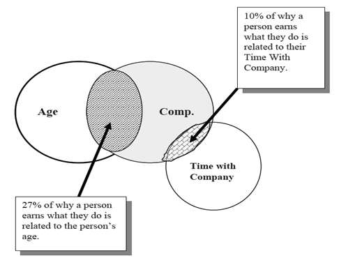
Notice that a person’s time with company holds only 10% responsible for his/her earning by profession. In other words, by adding this variable to our study, we improved our understanding of their compensation from 27% to 37%.
Therefore, we learnt, by using two variables rather than one, improved the ability to make accurate predictions about a person’s salary.
Things get much more complicated when your multiple independent variables are related to with each other. This phenomenon is known as Multicollinearity. This is undesirable. To avoid such situation, it is advisable to look for Variance Inflation Factor (VIF). For no multicollinearity, VIF should be ( VIF < 2). In case of high VIF, look for correlation table to find highly correlated variables and drop one of correlated ones.
Along with multi-collinearity, regression suffers from Autocorrelation, Heteroskedasticity.
In an multiple regression model, we try to predict
![]()
Here, b1, b2, b3 …bk are slopes for each independent variables X1, X2, X3….Xk and a is intercept.
Example: Net worth = a+ b1 (Age) +b2 (Time with company)
How to implement regression in Python and R?
Linear regression has commonly known implementations in R packages and Python scikit-learn. Let’s look at the code of loading linear regression model in R and Python below:
Python Code
R Code
#Load Train and Test datasets
#Identify feature and response variable(s) and values must be numeric
x_train <- input_variables_values_training_datasets
y_train <- target_variables_values_training_datasets
x_test <- input_variables_values_test_datasets
x <- cbind(x_train,y_train)
# Train the model using the training sets and check score
linear <- lm(y_train ~ ., data = x)
summary(linear)
#Predict Output
predicted= predict(linear,x_test)
End Notes
In this article, we looked at linear regression from basics followed by methods to find best fit line, evaluation metric, multi-variate regression and methods to implement in python and R. If you are new to data science, I’d recommend you to master this algorithm, before proceeding to the higher ones.
Did you find this article helpful? Please share your opinions / thoughts in the comments section below.
If you like what you just read & want to continue your analytics learning, subscribe to our emails, follow us on twitter or like our facebook page.
I am a Business Analytics and Intelligence professional with deep experience in the Indian Insurance industry. I have worked for various multi-national Insurance companies in last 7 years.