Introduction
Python is fast becoming the preferred language in data science – and for good reason(s). It provides the larger ecosystem of a programming language and the depth of good scientific computation libraries. If you are starting to learn Python, have a look at learning path on Python.
Among its scientific computation libraries, I found Pandas to be the most useful for data science operations. Pandas, along with Scikit-learn provides almost the entire stack needed by a data scientist. This article focuses on providing 12 ways for data manipulation in Python. I’ve also shared some tips & tricks which will allow you to work faster.
I would recommend that you look at the codes for data exploration before going ahead. To help you understand better, I’ve taken a data set to perform these operations and manipulations.
If you’re just starting out your data science journey, you’ll love the ‘Introduction to Data Science‘ course. It covers the basics of Python, comprehensive introduction to statistics and several machine learning algorithms. A must-have course!
Data Set: I’ve used the data set of Loan Prediction problem. Download the dataset and get started.
Let’s get started
I’ll start by importing the Pandas module and loading the data set into Python environment as Pandas Dataframe:
import pandas as pd
import numpy as np
data = pd.read_csv("train.csv", index_col="Loan_ID")
#1 – Boolean Indexing in Pandas
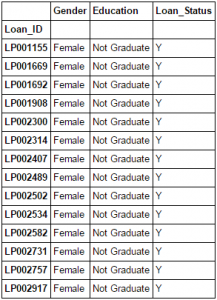
What do you do, if you want to filter values of a column based on conditions from another set of columns from a Pandas Dataframe? For instance, we want a list of all females who are not graduates and got a loan. Boolean indexing can help here. You can use the following code:
data.loc[(data["Gender"]=="Female") & (data["Education"]=="Not Graduate") & (data["Loan_Status"]=="Y"), ["Gender","Education","Loan_Status"]]
Read More about Boolean Indexing in Pandas here: Pandas Selecting and Indexing
#2 – Apply Function in Pandas
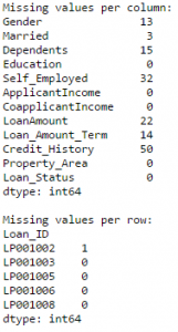
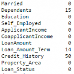
It is one of the commonly used Pandas functions for manipulating a pandas dataframe and creating new variables. Pandas Apply function returns some value after passing each row/column of a data frame with some function. The function can be both default or user-defined. For instance, here it can be used to find the #missing values in each row and column.
#Create a new function:
def num_missing(x):
  return sum(x.isnull())

#Applying per column:
print "Missing values per column:"
print data.apply(num_missing, axis=0) #axis=0 defines that function is to be applied on each column

#Applying per row:
print "\nMissing values per row:"
print data.apply(num_missing, axis=1).head() #axis=1 defines that function is to be applied on each row
Thus we get the desired result.
Note: Pandas head() function is used in second output because it contains many rows.
Read More about Pandas Apply here: Pandas Reference (apply)
#3 – Imputing missing values using Pandas
‘fillna()’ does it in one go. It is used for updating missing values with the overall mean/mode/median of the column. Let’s impute the ‘Gender’, ‘Married’ and ‘Self_Employed’ columns with their respective modes.
#First we import scipy function to determine the mode
from scipy.stats import mode
mode(data['Gender'])
Output: ModeResult(mode=array([‘Male’], dtype=object), count=array([489]))
This returns both mode and count. Remember that mode can be an array as there can be multiple values with high frequency. We will take the first one by default always using:
mode(data['Gender']).mode[0]
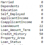
Now we can fill the missing values in the Pandas Dataframe data and check using technique #2.
#Impute the values:
data['Gender'].fillna(mode(data['Gender']).mode[0], inplace=True)
data['Married'].fillna(mode(data['Married']).mode[0], inplace=True)
data['Self_Employed'].fillna(mode(data['Self_Employed']).mode[0], inplace=True)

#Now check the #missing values again to confirm:
print data.apply(num_missing, axis=0)
Hence, it is confirmed that missing values in Pandas dataframe are imputed. Please note that this is the most primitive form of imputation. Other sophisticated techniques include modeling the missing values, using grouped averages (mean/mode/median). I’ll cover that part in my next articles.
Read More about imputing missing values in Pandas dataframe here: Pandas Reference (fillna)
#4 – Pivot Table in Pandas
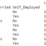
Pandas can be used to create MS Excel style pivot tables. For instance, in this case, a key column is “LoanAmount” which has missing values. We can impute it using mean amount of each ‘Gender’, ‘Married’ and ‘Self_Employed’ group. The mean ‘LoanAmount’ of each group in Pandas dataframe can be determined as:
#Determine pivot table
impute_grps = data.pivot_table(values=["LoanAmount"], index=["Gender","Married","Self_Employed"], aggfunc=np.mean)
print impute_grps
Read more about Pandas Pivot Table here: Pandas Reference (Pivot Table)
#5 – Multi-Indexing in Pandas Dataframe
If you notice the output of step #3, it has a strange property. Each Pandas index is made up of a combination of 3 values. This is called Multi-Indexing. It helps in performing operations really fast.
Continuing the example from #3, we have the values for each group but they have not been imputed.
This can be done using the various techniques from pandas learned till now.
#iterate only through rows with missing LoanAmount
for i,row in data.loc[data['LoanAmount'].isnull(),:].iterrows():
  ind = tuple([row['Gender'],row['Married'],row['Self_Employed']])
  data.loc[i,'LoanAmount'] = impute_grps.loc[ind].values[0]

#Now check the #missing values again to confirm:
print data.apply(num_missing, axis=0)
Note:
- Multi-index requires tuple for defining groups of indices in pandas loc statement. This is a tuple used in function.
- The .values[0] suffix is required because, by default a series element is returned which has an index not matching with that of the pandas dataframe. In this case, a direct assignment gives an error.
#6. Pandas Crosstab
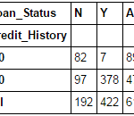
This function is used to get an initial “feel” (view) of the data. Here, we can validate some basic hypothesis. For instance, in this case, “Credit_History” is expected to affect the loan status significantly. This can be tested using cross-tabulation as shown below:
pd.crosstab(data["Credit_History"],data["Loan_Status"],margins=True)
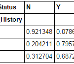
These are absolute numbers. But, percentages can be more intuitive in making some quick insights. We can do this using the Pandas apply function:
def percConvert(ser):
  return ser/float(ser[-1])
  pd.crosstab(data["Credit_History"],data["Loan_Status"],margins=True).apply(percConvert, axis=1)
Now, it is evident that people with a credit history have much higher chances of getting a loan as 80% people with credit history got a loan as compared to only 9% without credit history.
But that’s not it. It tells an interesting story. Since I know that having a credit history is super important, what if I predict loan status to be Y for ones with credit history and N otherwise. Surprisingly, we’ll be right 82+378=460 times out of 614 which is a whopping 75%!
I won’t blame you if you’re wondering why the hell do we need statistical models. But trust me, increasing the accuracy by even 0.001% beyond this mark is a challenging task. Would you take this challenge?
Note: 75% is on train set. The test set will be slightly different but close. Also, I hope this gives some intuition into why even a 0.05% increase in accuracy can result in jump of 500 ranks on the Kaggle leaderboard.
Read More about Pandas Crosstab function here: Pandas Reference (crosstab)
#7 – Merge Pandas DataFrames
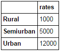
Merging Pandas dataframes become essential when we have information coming from different sources to be collated. Consider a hypothetical case where the average property rates (INR per sq meters) is available for different property types. Let’s define a Pandas dataframe as:
prop_rates = pd.DataFrame([1000, 5000, 12000], index=['Rural','Semiurban','Urban'],columns=['rates'])
prop_rates
Now we can merge this information with the original Pandas dataframe as:
data_merged = data.merge(right=prop_rates, how='inner',left_on='Property_Area',right_index=True, sort=False)
data_merged.pivot_table(values='Credit_History',index=['Property_Area','rates'], aggfunc=len)
The pivot table validates successful merge operation. Note that the ‘values’ argument is irrelevant here because we are simply counting the values.
ReadMore: Pandas Reference (merge)
#8 – Sorting Pandas DataFrames
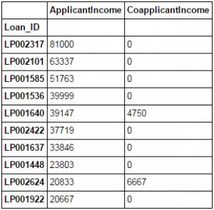
Pandas allow easy sorting based on multiple columns. This can be done as:
data_sorted = data.sort_values(['ApplicantIncome','CoapplicantIncome'], ascending=False)
data_sorted[['ApplicantIncome','CoapplicantIncome']].head(10)
Note: Pandas “sort” function is now deprecated. We should use “sort_values” instead.
More: Pandas Reference (sort_values)
#9 – Plotting (Boxplot & Histogram) with Pandas
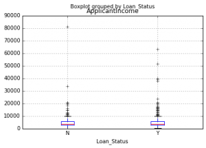
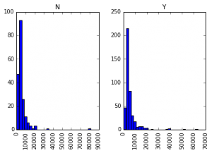
Many of you might be unaware that boxplots and histograms can be directly plotted in Pandas and calling matplotlib separately is not necessary. It’s just a 1-line command. For instance, if we want to compare the distribution of ApplicantIncome by Loan_Status:
import matplotlib.pyplot as plt
%matplotlib inline
data.boxplot(column="ApplicantIncome",by="Loan_Status")
data.hist(column="ApplicantIncome",by="Loan_Status",bins=30)
This shows that income is not a big deciding factor on its own as there is no appreciable difference between the people who received and were denied the loan.
Read More about Pandas Histogram & Pandas Boxplot here: Pandas Reference (hist) | Pandas Reference (boxplot)
#10 – Cut function for binning
Sometimes numerical values make more sense if clustered together. For example, if we’re trying to model traffic (#cars on road) with time of the day (minutes). The exact minute of an hour might not be that relevant for predicting traffic as compared to actual period of the day like “Morning”, “Afternoon”, “Evening”, “Night”, “Late Night”. Modeling traffic this way will be more intuitive and will avoid overfitting.
Here we define a simple function which can be re-used for binning any variable fairly easily.
#Binning:
def binning(col, cut_points, labels=None):
  #Define min and max values:
  minval = col.min()
  maxval = col.max()

  #create list by adding min and max to cut_points
  break_points = [minval] + cut_points + [maxval]

  #if no labels provided, use default labels 0 ... (n-1)
  if not labels:
    labels = range(len(cut_points)+1)

  #Binning using cut function of pandas
  colBin = pd.cut(col,bins=break_points,labels=labels,include_lowest=True)
  return colBin

#Binning age:
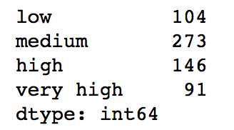
cut_points = [90,140,190]
labels = ["low","medium","high","very high"]
data["LoanAmount_Bin"] = binning(data["LoanAmount"], cut_points, labels)
print pd.value_counts(data["LoanAmount_Bin"], sort=False)
Read More about Pandas Cut Function here: Pandas Reference (cut)
#11 – Coding nominal data using Pandas
Often, we find a case where we’ve to modify the categories of a nominal variable. This can be due to various reasons:
- Some algorithms (like Logistic Regression) require all inputs to be numeric. So nominal variables are mostly coded as 0, 1….(n-1)
- Sometimes a category might be represented in 2 ways. For e.g. temperature might be recorded as “High”, “Medium”, “Low”, “H”, “low”. Here, both “High” and “H” refer to same category. Similarly, in “Low” and “low” there is only a difference of case. But, python would read them as different levels.
- Some categories might have very low frequencies and its generally a good idea to combine them.
Here I’ve defined a generic function which takes in input as a dictionary and codes the values using ‘replace’ function in Pandas.
#Define a generic function using Pandas replace function
def coding(col, codeDict):
  colCoded = pd.Series(col, copy=True)
  for key, value in codeDict.items():
    colCoded.replace(key, value, inplace=True)
  return colCoded

#Coding LoanStatus as Y=1, N=0:
print 'Before Coding:'
print pd.value_counts(data["Loan_Status"])
data["Loan_Status_Coded"] = coding(data["Loan_Status"], {'N':0,'Y':1})
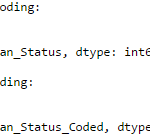
print '\nAfter Coding:'
print pd.value_counts(data["Loan_Status_Coded"])
Similar counts before and after proves the coding.
Read More about Pandas Replace Function here: Pandas Reference (replace)
#12 – Iterating over rows of a Pandas Dataframe
This is not a frequently used Pandas operation. Still, you don’t want to get stuck. Right? At times you may need to iterate through all rows of a Pandas dataframe using a for loop. For instance, one common problem we face is the incorrect treatment of variables in Python. This generally happens when:
- Nominal variables with numeric categories are treated as numerical.
- Numeric variables with characters entered in one of the rows (due to a data error) are considered categorical.
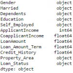
So it’s generally a good idea to manually define the column types. If we check the data types of all columns:
#Check current type:
data.dtypes
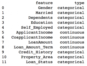
Here we see that Credit_History is a nominal variable but appearing as float. A good way to tackle such issues is to create a csv file with column names and types. This way, we can make a generic function to read the file and assign column data types. For instance, here I have created a csv file datatypes.csv.
#Load the file:
colTypes = pd.read_csv('datatypes.csv')
print colTypes
After loading this file, we can iterate through each row and assign the datatype using column ‘type’ to the variable name defined in the ‘feature’ column.
#Iterate through each row and assign variable type in a Pandas dataframe
#Note: astype is used to assign types

for i, row in colTypes.iterrows():  #i: dataframe index; row: each row in series format
    if row['type']=="categorical":
        data[row['feature']]=data[row['feature']].astype(np.object)
    elif row['type']=="continuous":
        data[row['feature']]=data[row['feature']].astype(np.float)
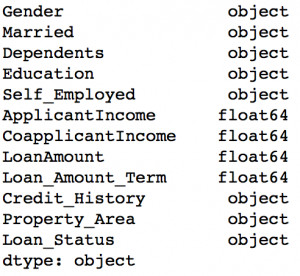
print data.dtypes
Now the credit history column is modified to ‘object’ type which is used for representing nominal variables in Pandas.
Read More about Pandas iterrows here: Pandas Reference (iterrows)
Projects
Now, its time to take the plunge and actually play with some other real datasets and test your learning in Pandas. So are you ready to take on the challenge? Accelerate your data science journey with the following Practice Problems:
 |
Practice Problem: Food Demand Forecasting Challenge | Predict the demand of meals for a meal delivery company |
 |
Practice Problem: HR Analytics Challenge | Identify the employees most likely to get promoted |
 |
Practice Problem: Predict Number of Upvotes | Predict number of upvotes on a query asked at an online question & answer platform |
End Notes
In this article, we covered various functions of Pandas which can make our life easy while performing data exploration and feature engineering. Also, we defined some generic functions which can be reused for achieving similar objective on different datasets.
Also See: If you have any doubts pertaining to Pandas or Python in general, feel free to discuss with us.
Did you find the article useful? Do you use some better (easier/faster) techniques for performing the tasks discussed above? Do you think there are better alternatives to Pandas in Python? We’ll be glad if you share your thoughts as comments below.


